Discovering Continuous Latent Space Representations for Graphs
Winston Yu, Jianming Geng, Barry Xue
UCSD Halıcıoğlu Data Science Institute
UC San Diego Data Science Senior Capstone Project
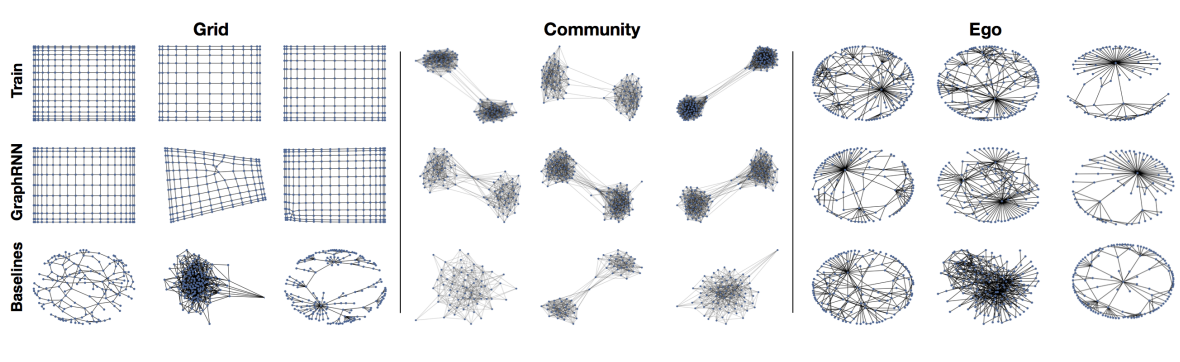
Figure 1: From "GraphRNN: Generating Realistic Graphs with Deep Auto-regressive Models"; Comparison between original graph (top row), generation from GraphRNN, a deep auto-regressive graph generation model (second row), and random generation baseline (bottom row).
Introduction
Graph neural networks (GNNs) have seen tremendous success in recent years, leading to their widespread adoption in a variety of applications. However, recent studies have demonstrated that GNNs can be vulnerable to adversarial attacks. Adversarial attacks allow adversaries to manipulate GNNs by introducing small, seemingly harmless perturbations to the input data, which can lead to misclassification or unexpected behavior from the GNN. Such attacks can have drastic impacts on security and privacy, particularly in safety-critical or privacy-sensitive applications. Consequently, research into adversarial attacks on GNNs is becoming increasingly important, and we thus propose an adversarial attack framework that discovers continuous latent representations of graphs to which adversarial modifications are added, instead of modifying a benign graph itself.
Background
1. Generating Attack with Surrogate Model
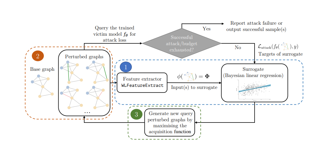
Figure 2: From "Adversarial Attacks on Graph Classification via Bayesian Optimisation"; a visualization of the attack generation procedure.
Generating Attack with Surrogate Model on Graphs is a method used to find the most effective attacks on graphs using machine learning algorithms. The main goal is to learn a surrogate model from the data of the graph, and then use the generated model to simulate attack scenarios and search for the most effective attack strategy. This technique can be especially useful for cyber-security applications, such as identifying potential weaknesses in networks or finding malicious pathways in a graph.
2. Generating Adversarial Example with WGAN
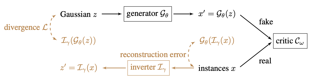
Figure 3: From "Generating Natural Adversarial Example"; A visualization of the Wasserstein GAN procedure.
This approach is a novel method for generating natural adversarial examples, which are inputs that can fool state-of-the-art machine learning models while being imperceptible to human observation. Its architecture is comprised of an inverter, which maps from the data space to the latent space, a generator, which is trained to be part of a Wasserstein GAN and maps from the latent space to the data space, and a search algorithm, which explores the latent space for representations of adversarial examples.
3. Graph2Vec
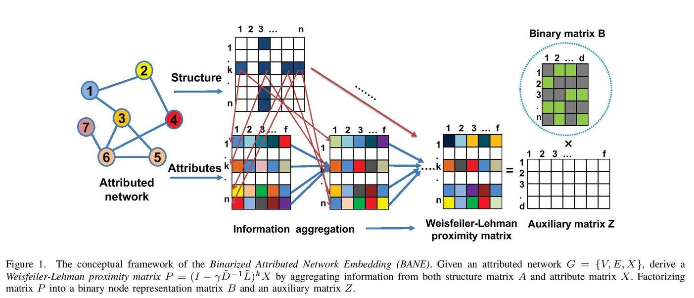
Figure 4: From "Generating Natural Adversarial Example"; A visualization of the Graph2Vec structure.
Graph2Vec is a machine learning method that embeds a graph of arbitrary size into Euclidean space. We intend to first pass graphs to Graph2Vec and then pass the resulting vectors to the inverter.
Our Proposal
Discriminator: MLP
Generator: GraphRNN
Inverter: Graph2Vec/GAM + MLP
Generator: GraphRNN
Figure 4: Structure of the GraphRNN model.
GraphRNN is an autoregressive graph generation model that uses two GRU recurrent neural networks. The first GRU model updates a hidden state, which is a representation of the graph that has been generated so far. The second GRU model takes the hidden state of the first GRU and uses it to generate adjacency vectors. Originally, the model was trained with binary cross entropy loss, comparing the generated edges and the ground truth. We propose to train the GraphRNN to minimize the Wasserstein distance between the data distribution and the distribution of GraphRNN.
Inverter & Discriminator: Multi-layer Perceptrons
The inverter and the discriminator are simple multi-layer perceptrons. For the inverter, we decided to first try to train Graph2Vec to generate embeddings, which would be passed to the inverter. However, we later found that the Graph2Vec implementation from the package “Karate Club” is not compatible with Torch’s gradient computation. Hence, we decided to switch to GAM (Graph Attention Model) as an embedding technique. However, GAM did not work either.
Overall Planned Structure
Figure 5.1: Structure of our attack generation procedure.
We divide our training algorithm into four parts in total: (1). Discriminator; (2). Generator; (3). Inverter; (4). Search Algorithm.
We first train the discriminator, which corresponds to the dark blue box in the figure above. The discriminator takes a graph as input and returns a scalar between -1 and 1. During the training of the discriminator, we freeze the parameters of all other models. The discriminator is trained to maximize its output for graphs from the dataset and to minimize its output for graphs generated by GraphRNN. Finally, to gauge how close the distribution of GraphRNN is to the true distribution, we take the difference between the expected value of the discriminator on the true dataset and the expected value of the discriminator on the generated graphs, which by the Kantorovich-Rubinstein duality is the Wasserstein distance.
We then train the generator, which corresponds to the dark green box in the figure. To train the generator, we first freeze the parameters of all other models and then sample a batch of noise from a normal distribution on the latent space. This noise is passed to the generator to generate a batch of fake graphs. The generator is then trained to maximize the output of the (frozen) discriminator because this decreases the Wasserstein distance between the true distribution and the generator’s distribution.
After that, we train the inverter, which corresponds to the red blocks from the image. A composition of a graph2vec model and a multi-layer perceptron, in that order, is what we call the inverter, whose domain is the space of graphs and whose codomain is the latent space of GraphRNN. The graph2vec model is pre-trained on the graphs produced by GraphRNN and on the graphs of the true distribution, and its weights are frozen hereafter. The inverter is trained to minimize the weighted sum of two distances: the standard Euclidean distance between an element in the latent space and the inverter’s output when given a graph generated from that element, and the Gromov-Wasserstein distance between a graph (either from the dataset or from GraphRNN) and GraphRNN’s output when given a latent element outputted by the inverter when the inverter’s argument is that graph.
What We Have Currently
Figure 5.2: Current structure of our attack generation procedure.
We were only able to train the discriminator and the generator due to time constraints. The discriminator is a weakened form of the originally planned one: instead of first passing graphs to a pre-trained graph2vec model, we merely pad flattened adjacency matrices to a common size and then feed it to a multi-layer perceptron.
Result of our Investigation
1. New Training Procedure for GraphRNN
Originally, GraphRNN is trained by comparing the generated padded adjacency vector with the sequenced original adjacency matrix using binary cross entropy loss. This isn't ideal for the WGAN training procedure, where the generator needs to be trained by the discriminator's output, which is no longer an adjacency matrix.
For our new training process for the GraphRNN, we revert the output of node-level and edge-level RNN models to batches of generated adjacency matrices; then we pass these adjacency matrices into the discriminator network, whose output is used in our Wasserstein loss function. We will use this loss to update the node-level and edge-level RNN model parameters.
2. Observation on the three Losses
With our proposed WGAN training regime, we trained the generator, the discriminator, and the inverter, all in one training loop. We recorded the loss of each of the models every epoch.
Figure 6: Comparison of Graph2Vec Embedding between Real Graphs and Generated Graphs.
We found that as the discriminator loss improves overtime, the generator loss and inverter loss quickly hits a threshold and cannot improve further beyond this point. This can be an indication that the new training regime isn't suitable for GraphRNN training, and the quality of our generated graphs is not good enough support the training of the discriminator and inverter.
Challenges
1. Previous work and time constraint
There isn’t much research done in generating latent representations of adversarial examples, especially not for the task of attacking graph classifiers, so we had to implement our ideas from the ground up. Also, the time frame for this project is 10 weeks, which is very little time to fully develop this framework and run experiments.
2. GraphRNN output during training is difficult to interpret and process by the discriminator
The output of GraphRNN is a graph of almost arbitrary size. However, in practice, the GraphRNN implementation returned batched and packed versions of the original graph adjacency vector, which made every version of the discriminator fail to compute.
3. Lack of networkx integration in PyTorch/PyTorch Geometric
The procedure of computing high-quality graph features (e.g. clustering coefficient) is too complex for us to implement with solely PyTorch functions, so we relied on NetworkX functions to do these computations. This became an issue during the training of GraphRNN because NetworkX functions are incompatible with the way PyTorch computes gradients, which means that gradient descent cannot happen. We resorted to using a simple multi-layer perceptron as our discriminator, which takes as input flattened and padded adjacency matrices, but flattening and padding adjacency matrix loses structural information.
Future Plan
If we continue this research project, we want to do the following:
1. Improve implementation of GraphRNN
Due to a lack of time, we did not thoroughly investigate the GraphRNN implementation and treated the model as a black box. We encountered many issues related to loading the data, model training, and graph generation using the official implementation. As we were troubleshooting the model, we noticed that the implementation is incompatible with downstream processing of GraphRNN outputs. We would have liked more time to edit GraphRNN’s implementation to be more compatible with other tasks.
2. Use a graph classifier as our discriminator instead of a simple multi-layer perceptron
Currently, the discriminator is a simple MLP that takes in flattened and padded adjacency matrices. The discriminator is trained by the negative Wasserstein distance between the generated distribution and the real data distribution. However, because reshaping adjacency matrices caused a loss of structural information, we would have preferred to use a model that could process a graph without reshaping operations.
After evaluating the result of the current setup, we think a simple MLP can't take into account specific graph properties, and thus cannot accurately discern between the two distributions. We propose to substitute this MLP with a Graph Attention Machine (GAM) classifier, because GAM can utilize the Weisfeiler-Lehman kernel to capture graph features to discern between the real and the generated distributions. Ideally, this will provide high quality loss for the discriminator training and the generator training.
Reference
- GraphRNN: Paper, Original Implementation
- Attack on GNN with Bayesian Optimization: Paper, Original Implementation
- Wasserstein GAN: Paper, Original Implementation
- Graph Attention Model: Paper, Original Implementation